automl

Alex Boulangé

january 16, 2020

Contents

 0.1 Introduction to automl package
 0.2 Why & how automl
  0.2.1 Deep Learning existing frameworks, disadvantages
  0.2.2 Neural Network - Deep Learning, disadvantages
  0.2.3 Metaheuristic - PSO, benefits
  0.2.4 Birth of automl package
  0.2.5 Mix 1: hyperparameters tuning with PSO
  0.2.6 Mix 2: PSO instead of gradient descent
 0.3 First steps: How to
  0.3.1 fit a regression model manually (hard way)
  0.3.2 fit a regression model automatically (easy way, Mix 1)
  0.3.3 fit a regression model experimentally (experimental way, Mix 2)
  0.3.4 fit a regression model with custom cost (experimental way, Mix 2)
  0.3.5 fit a classification model with softmax (Mix 2)
  0.3.6 change the model parameters (shape …)
  0.3.7 continue training on saved model (fine tuning …)
  0.3.8 use the 2 steps automatic approach
 0.4 ToDo List

0.1 Introduction to automl package

This document is intended to answer the following questions; why & how automl and how to use it

automl package provides:
-Deep Learning last tricks (those who have taken Andrew NG’s MOOC on Coursera will be in familiar territory)
-hyperparameters autotune with metaheuristic (PSO)
-experimental stuff and more to come (you’re welcome as coauthor!)

0.2 Why & how automl

0.2.1 Deep Learning existing frameworks, disadvantages

Deploying and maintaining most Deep Learning frameworks means: Python…
R language is so simple to install and maintain in production environments that it is obvious to use a pure R based package for deep learning !

0.2.2 Neural Network - Deep Learning, disadvantages

Disadvantages :
1st disadvantage: you have to test manually different combinations of parameters (number of layers, nodes, activation function, etc …) and then also tune manually hyper parameters for training (learning rate, momentum, mini batch size, etc …)
2nd disadvantage: only for those who are not mathematicians, calculating derivative in case of new cost or activation function, may by an issue.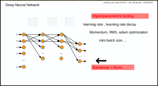

0.2.3 Metaheuristic - PSO, benefits

The Particle Swarm Optimization algorithm is a great and simple one.
In a few words, the first step consists in throwing randomly a set of particles in a space and the next steps consist in discovering the best solution while converging.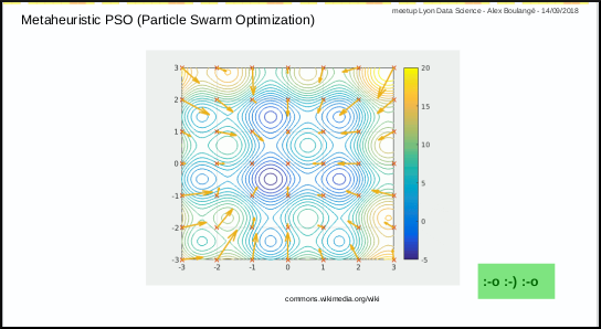

video tutorial from Yarpiz is a great ressource

0.2.4 Birth of automl package

automl package was born from the idea to use metaheuristic PSO to address the identified disadvantages above.
And last but not the least reason: use R and R only :-)
3 functions are available:
- automl_train_manual: the manual mode to train a model
- automl_train: the automatic mode to train model
- automl_predict: the prediction function to apply a trained model on datas

0.2.5 Mix 1: hyperparameters tuning with PSO

Mix 1 consists in using PSO algorithm to optimize the hyperparameters: each particle corresponds to a set of hyperparameters.
The automl_train function was made to do that.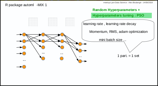

0.2.6 Mix 2: PSO instead of gradient descent

Mix 2 is experimental, it consists in using PSO algorithm to optimize the weights of Neural Network in place of gradient descent: each particle corresponds to a set of neural network weights matrices.
The automl_train_manual function do that too.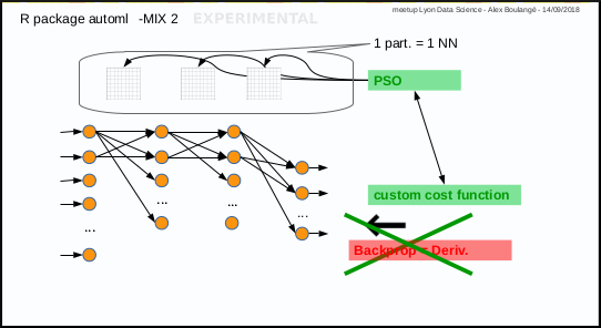

0.3 First steps: How to

For those who will laugh at seeing deep learning with one hidden layer and the Iris data set of 150 records, I will say: you’re perfectly right :-)
The goal at this stage is simply to take the first steps

0.3.1 fit a regression model manually (hard way)

Subject: predict Sepal.Length given other Iris parameters
1st with gradient descent and default hyperparameters value for learning rate (0.001) and mini batch size (32)

data(iris)
xmat <- cbind(iris[,2:4], as.numeric(iris$Species))
ymat <- iris[,1]
amlmodel <- automl_train_manual(Xref = xmat, Yref = ymat)

## (cost: mse)
## cost epoch10: 0.805238955644501 (cv cost: 4.21618247893937) (LR:  0.001 ) 
## cost epoch20: 0.635110258608589 (cv cost: 1.6721782273314) (LR:  0.001 ) 
## cost epoch30: 0.442896887636891 (cv cost: 1.38613208757511) (LR:  0.001 ) 
## cost epoch40: 0.417861223304396 (cv cost: 1.14304235928791) (LR:  0.001 ) 
## cost epoch50: 0.384222897412199 (cv cost: 0.959845846511371) (LR:  0.001 ) 
##    dim X: [4,135]
##    dim W1: [10,4] (min|max: -1.54429770594677, 1.76673847197307)
##    dim bB1: [10,1] (min|max: 0, 0.545298555899576)
##    dim W2: [1,10] (min|max: -0.0130920429820853, 0.349457454208908)
##    dim bB2: [1,1] (min|max: 0.074428956661853, 0.074428956661853)
##    dim Y: [1,135]

res <- cbind(ymat, automl_predict(model = amlmodel, X = xmat))
colnames(res) <- c('actual', 'predict')
head(res)

##      actual  predict
## [1,]    5.1 3.040397
## [2,]    4.9 2.885246
## [3,]    4.7 2.911639
## [4,]    4.6 2.951945
## [5,]    5.0 3.071427
## [6,]    5.4 3.365510

:-[] no pain, no gain …
After some manual fine tuning on learning rate, mini batch size and iterations number (epochs):

data(iris)
xmat <- cbind(iris[,2:4], as.numeric(iris$Species))
ymat <- iris[,1]
amlmodel <- automl_train_manual(Xref = xmat, Yref = ymat,
                                hpar = list(learningrate = 0.01,
                                minibatchsize = 2^2,
                                numiterations = 30))

## (cost: mse)
## cost epoch10: 0.07483378655409 (cv cost: 0.466478285718589) (LR:  0.01 ) 
## cost epoch20: 0.275546796158403 (cv cost: 0.294895895020273) (LR:  0.01 ) 
## cost epoch30: 0.231827727788502 (cv cost: 0.233179461368555) (LR:  0.01 ) 
##    dim X: [4,135]
##    dim W1: [10,4] (min|max: -1.54429770594677, 2.73130744979701)
##    dim bB1: [10,1] (min|max: -0.317658298585351, 1.99139261324871)
##    dim W2: [1,10] (min|max: -0.313978049365135, 0.286454921099375)
##    dim bB2: [1,1] (min|max: 0.337210920487028, 0.337210920487028)
##    dim Y: [1,135]

res <- cbind(ymat, automl_predict(model = amlmodel, X = xmat))
colnames(res) <- c('actual', 'predict')
head(res)

##      actual  predict
## [1,]    5.1 5.662462
## [2,]    4.9 5.112758
## [3,]    4.7 5.319313
## [4,]    4.6 5.236026
## [5,]    5.0 5.772403
## [6,]    5.4 6.152288

Better result, but with human efforts!

0.3.2 fit a regression model automatically (easy way, Mix 1)

Same subject: predict Sepal.Length given other Iris parameters

data(iris)
xmat <- as.matrix(cbind(iris[,2:4], as.numeric(iris$Species)))
ymat <- iris[,1]
start.time <- Sys.time()
amlmodel <- automl_train(Xref = xmat, Yref = ymat,
                         autopar = list(psopartpopsize = 15,
                                        numiterations = 5,
                                        auto_layers_max = 1,
                                        nbcores = 4))

## (cost: mse)
## iteration 1 particle 1 weighted err: 16.07611 (train: 15.72634 cvalid: 14.85191 ) BEST MODEL KEPT
## iteration 1 particle 2 weighted err: 16.3075 (train: 15.87959 cvalid: 14.80982 )
## iteration 1 particle 3 weighted err: 16.94757 (train: 16.49087 cvalid: 15.34912 )
## iteration 1 particle 4 weighted err: 20.13882 (train: 19.37989 cvalid: 17.48256 )
## iteration 1 particle 5 weighted err: 14.5494 (train: 14.31557 cvalid: 13.731 ) BEST MODEL KEPT
## iteration 1 particle 6 weighted err: 19.092 (train: 18.42356 cvalid: 16.75247 )
## iteration 1 particle 7 weighted err: 12.88628 (train: 12.82588 cvalid: 12.67488 ) BEST MODEL KEPT
## iteration 1 particle 8 weighted err: 9.66599 (train: 8.34742 cvalid: 9.17153 ) BEST MODEL KEPT
## iteration 1 particle 9 weighted err: 12.87134 (train: 12.85174 cvalid: 12.80274 )
## iteration 1 particle 10 weighted err: 0.53282 (train: 0.51617 cvalid: 0.47454 ) BEST MODEL KEPT
## iteration 1 particle 11 weighted err: 6.02654 (train: 2.92766 cvalid: 4.86446 )
## iteration 1 particle 12 weighted err: 20.07748 (train: 19.32307 cvalid: 17.43702 )
## iteration 1 particle 13 weighted err: 0.8172 (train: 0.3341 cvalid: 0.63604 )
## iteration 1 particle 14 weighted err: 15.12864 (train: 14.84328 cvalid: 14.12987 )
## iteration 1 particle 15 weighted err: 16.04961 (train: 15.68522 cvalid: 14.77424 )
## iteration 2 particle 1 weighted err: 3.25095 (train: 0.44164 cvalid: 2.19746 )
## iteration 2 particle 2 weighted err: 6.72649 (train: 4.47423 cvalid: 5.88189 )
## iteration 2 particle 3 weighted err: 1.5405 (train: 0.07335 cvalid: 0.99032 )
## iteration 2 particle 4 weighted err: 7.84113 (train: 4.75334 cvalid: 6.68321 )
## iteration 2 particle 5 weighted err: 0.34593 (train: 0.27883 cvalid: 0.11109 ) BEST MODEL KEPT
## iteration 2 particle 6 weighted err: 12.3852 (train: 12.32275 cvalid: 12.1666 )
## iteration 2 particle 7 weighted err: 0.72669 (train: 0.40974 cvalid: 0.60783 )
## iteration 2 particle 8 weighted err: 9.46709 (train: 7.63313 cvalid: 8.77935 )
## iteration 2 particle 9 weighted err: 0.26449 (train: 0.21547 cvalid: 0.0929 ) BEST MODEL KEPT
## iteration 2 particle 10 weighted err: 0.53108 (train: 0.50309 cvalid: 0.52058 )
## iteration 2 particle 11 weighted err: 0.21346 (train: 0.18145 cvalid: 0.10142 ) BEST MODEL KEPT
## iteration 2 particle 12 weighted err: 10.01845 (train: 7.41695 cvalid: 9.04289 )
## iteration 2 particle 13 weighted err: 0.8172 (train: 0.3341 cvalid: 0.63604 )
## iteration 2 particle 14 weighted err: 11.38494 (train: 10.64396 cvalid: 11.10707 )
## iteration 2 particle 15 weighted err: 0.65022 (train: 0.48874 cvalid: 0.58967 )
## iteration 3 particle 1 weighted err: 0.16991 (train: 0.14985 cvalid: 0.0997 ) BEST MODEL KEPT
## iteration 3 particle 2 weighted err: 0.2571 (train: 0.20501 cvalid: 0.07478 )
## iteration 3 particle 3 weighted err: 0.21233 (train: 0.17727 cvalid: 0.08962 )
## iteration 3 particle 4 weighted err: 0.27683 (train: 0.22695 cvalid: 0.10223 )
## iteration 3 particle 5 weighted err: 0.29569 (train: 0.23231 cvalid: 0.07386 )
## iteration 3 particle 6 weighted err: 5.28776 (train: 2.08285 cvalid: 4.08592 )
## iteration 3 particle 7 weighted err: 0.3073 (train: 0.23883 cvalid: 0.06767 )
## iteration 3 particle 8 weighted err: 0.26232 (train: 0.22815 cvalid: 0.24951 )
## iteration 3 particle 9 weighted err: 0.26025 (train: 0.20627 cvalid: 0.07132 )
## iteration 3 particle 10 weighted err: 0.53108 (train: 0.50309 cvalid: 0.52058 )
## iteration 3 particle 11 weighted err: 0.21346 (train: 0.18145 cvalid: 0.10142 )
## iteration 3 particle 12 weighted err: 0.46891 (train: 0.41581 cvalid: 0.28306 )
## iteration 3 particle 13 weighted err: 0.17794 (train: 0.15515 cvalid: 0.09818 )
## iteration 3 particle 14 weighted err: 2.70264 (train: 0.22617 cvalid: 1.77397 )
## iteration 3 particle 15 weighted err: 0.13619 (train: 0.12791 cvalid: 0.10723 ) BEST MODEL KEPT
## iteration 4 particle 1 weighted err: 0.16991 (train: 0.14985 cvalid: 0.0997 )
## iteration 4 particle 2 weighted err: 0.2571 (train: 0.20501 cvalid: 0.07478 )
## iteration 4 particle 3 weighted err: 0.21233 (train: 0.17727 cvalid: 0.08962 )
## iteration 4 particle 4 weighted err: 0.16451 (train: 0.14885 cvalid: 0.1097 )
## iteration 4 particle 5 weighted err: 0.1932 (train: 0.16253 cvalid: 0.08585 )
## iteration 4 particle 6 weighted err: 0.33533 (train: 0.27301 cvalid: 0.1172 )
## iteration 4 particle 7 weighted err: 0.26357 (train: 0.20933 cvalid: 0.07372 )
## iteration 4 particle 8 weighted err: 0.25709 (train: 0.20479 cvalid: 0.07402 )
## iteration 4 particle 9 weighted err: 0.26025 (train: 0.20627 cvalid: 0.07132 )
## iteration 4 particle 10 weighted err: 0.52717 (train: 0.50699 cvalid: 0.45654 )
## iteration 4 particle 11 weighted err: 0.12243 (train: 0.11719 cvalid: 0.1041 ) BEST MODEL KEPT
## iteration 4 particle 12 weighted err: 0.31195 (train: 0.25553 cvalid: 0.1145 )
## iteration 4 particle 13 weighted err: 0.17794 (train: 0.15515 cvalid: 0.09818 )
## iteration 4 particle 14 weighted err: 0.28483 (train: 0.22989 cvalid: 0.09254 )
## iteration 4 particle 15 weighted err: 0.13619 (train: 0.12791 cvalid: 0.10723 )
## iteration 5 particle 1 weighted err: 0.15756 (train: 0.14336 cvalid: 0.10787 )
## iteration 5 particle 2 weighted err: 0.14906 (train: 0.13677 cvalid: 0.10603 )
## iteration 5 particle 3 weighted err: 0.19496 (train: 0.16397 cvalid: 0.08648 )
## iteration 5 particle 4 weighted err: 0.16451 (train: 0.14885 cvalid: 0.1097 )
## iteration 5 particle 5 weighted err: 0.15987 (train: 0.1455 cvalid: 0.1096 )
## iteration 5 particle 6 weighted err: 0.23285 (train: 0.19629 cvalid: 0.10489 )
## iteration 5 particle 7 weighted err: 0.15237 (train: 0.13932 cvalid: 0.10669 )
## iteration 5 particle 8 weighted err: 0.14906 (train: 0.1377 cvalid: 0.10931 )
## iteration 5 particle 9 weighted err: 0.12347 (train: 0.11734 cvalid: 0.10201 )
## iteration 5 particle 10 weighted err: 0.47067 (train: 0.42237 cvalid: 0.3016 )
## iteration 5 particle 11 weighted err: 0.12243 (train: 0.11719 cvalid: 0.1041 )
## iteration 5 particle 12 weighted err: 0.22751 (train: 0.19169 cvalid: 0.10214 )
## iteration 5 particle 13 weighted err: 0.10348 (train: 0.10208 cvalid: 0.09857 ) BEST MODEL KEPT
## iteration 5 particle 14 weighted err: 0.17735 (train: 0.15256 cvalid: 0.09059 )
## iteration 5 particle 15 weighted err: 0.13619 (train: 0.12791 cvalid: 0.10723 )

end.time <- Sys.time()
cat(paste('time ellapsed:', end.time - start.time, '\n'))

## time ellapsed: 1.63398174842199

res <- cbind(ymat, automl_predict(model = amlmodel, X = xmat))
colnames(res) <- c('actual', 'predict')
head(res)

##      actual  predict
## [1,]    5.1 5.042245
## [2,]    4.9 4.611002
## [3,]    4.7 4.731076
## [4,]    4.6 4.749674
## [5,]    5.0 5.128494
## [6,]    5.4 5.483997

It’s even better, with no human efforts but machine time
Windows users won’t benefit from parallelization, the function uses parallel package included with R base…

0.3.3 fit a regression model experimentally (experimental way, Mix 2)

Same subject: predict Sepal.Length given other Iris parameters

data(iris)
xmat <- as.matrix(cbind(iris[,2:4], as.numeric(iris$Species)))
ymat <- iris[,1]
amlmodel <- automl_train_manual(Xref = xmat, Yref = ymat,
                                hpar = list(modexec = 'trainwpso',
                                            numiterations = 30,
                                            psopartpopsize = 50))

## (cost: mse)
## cost epoch10: 0.0827230804228524 (cv cost: 0.0905949933685151) (LR:  0 ) 
## cost epoch20: 0.0742651449342831 (cv cost: 0.0820428875464537) (LR:  0 ) 
## cost epoch30: 0.073268785428924 (cv cost: 0.0759160345752076) (LR:  0 ) 
##    dim X: [4,135]
##    dim W1: [10,4] (min|max: -5.71510122702586, 9.43334015646581)
##    dim bB1: [10,1] (min|max: -0.139628718730307, 0.0615382424233414)
##    dim W2: [1,10] (min|max: -0.0537321480169208, 0.32227090072508)
##    dim bB2: [1,1] (min|max: 0.066365884761476, 0.066365884761476)
##    dim Y: [1,135]

res <- cbind(ymat, automl_predict(model = amlmodel, X = xmat))
colnames(res) <- c('actual', 'predict')
head(res)

##      actual  predict
## [1,]    5.1 5.065030
## [2,]    4.9 4.469249
## [3,]    4.7 4.649156
## [4,]    4.6 4.646810
## [5,]    5.0 5.184187
## [6,]    5.4 5.692447

Pretty good too, even better!

0.3.4 fit a regression model with custom cost (experimental way, Mix 2)

Same subject: predict Sepal.Length given other Iris parameters
Let’s try with Mean Absolute Percentage Error instead of Mean Square Error

data(iris)
xmat <- as.matrix(cbind(iris[,2:4], as.numeric(iris$Species)))
ymat <- iris[,1]
f <- 'J=abs((y-yhat)/y)'
f <- c(f, 'J=sum(J[!is.infinite(J)],na.rm=TRUE)')
f <- c(f, 'J=(J/length(y))')
f <- paste(f, collapse = ';')
amlmodel <- automl_train_manual(Xref = xmat, Yref = ymat,
                                hpar = list(modexec = 'trainwpso',
                                            numiterations = 30,
                                            psopartpopsize = 50,
                                            costcustformul = f))

## (cost: custom)
## cost epoch10: 0.0641352199927726 (cv cost: 0.0541888618566213) (LR:  0 ) 
## cost epoch20: 0.0582926167466713 (cv cost: 0.0523653406107709) (LR:  0 ) 
## cost epoch30: 0.0573700514993968 (cv cost: 0.0535607803292487) (LR:  0 ) 
##    dim X: [4,135]
##    dim W1: [10,4] (min|max: -9.05531100347454, 2.26590853900144)
##    dim bB1: [10,1] (min|max: -0.0601253304054113, 0.0399524442723589)
##    dim W2: [1,10] (min|max: -0.0292102857934989, 0.538940524656712)
##    dim bB2: [1,1] (min|max: 0.00164941620007934, 0.00164941620007934)
##    dim Y: [1,135]

res <- cbind(ymat, automl_predict(model = amlmodel, X = xmat))
colnames(res) <- c('actual', 'predict')
head(res)

##      actual  predict
## [1,]    5.1 5.056738
## [2,]    4.9 4.447762
## [3,]    4.7 4.639456
## [4,]    4.6 4.622778
## [5,]    5.0 5.177504
## [6,]    5.4 5.695871

0.3.5 fit a classification model with softmax (Mix 2)

Subject: predict Species given other Iris parameters
Softmax is available with PSO, no derivative needed ;-)

data(iris)
xmat = iris[,1:4]
lab2pred <- levels(iris$Species)
lghlab <- length(lab2pred)
iris$Species <- as.numeric(iris$Species)
ymat <- matrix(seq(from = 1, to = lghlab, by = 1), nrow(xmat), lghlab, byrow = TRUE)
ymat <- (ymat == as.numeric(iris$Species)) + 0
amlmodel <- automl_train_manual(Xref = xmat, Yref = ymat,
                                hpar = list(modexec = 'trainwpso',
                                layersshape = c(10, 0),
                                layersacttype = c('relu', 'softmax'),
                                layersdropoprob = c(0, 0),
                                numiterations = 50,
                                psopartpopsize = 50))

## (cost: crossentropy)
## cost epoch10: 0.870236074020942 (cv cost: 0.538739272849298) (LR:  0 ) 
## cost epoch20: 0.757282033049055 (cv cost: 0.512634130927213) (LR:  0 ) 
## cost epoch30: 0.665336489286255 (cv cost: 0.405940640471504) (LR:  0 ) 
## cost epoch40: 0.436565442235112 (cv cost: 0.304221712919552) (LR:  0 ) 
## cost epoch50: 0.396825986932571 (cv cost: 0.28317967654653) (LR:  0 ) 
##    dim X: [4,135]
##    dim W1: [10,4] (min|max: -10, 10)
##    dim bB1: [10,1] (min|max: -0.791357447569002, 0.935502029600105)
##    dim W2: [3,10] (min|max: -0.113304196183761, 3.64390040008716)
##    dim bB2: [3,1] (min|max: -0.711577511465429, 0.00524904114168052)
##    dim Y: [3,135]

res <- cbind(ymat, automl_predict(model = amlmodel, X = xmat))
colnames(res) <- c(paste('act',lab2pred, sep = '_'),
paste('pred',lab2pred, sep = '_'))
head(res)

##   act_setosa act_versicolor act_virginica pred_setosa pred_versicolor
## 1          1              0             0   1.0000000    8.642711e-09
## 2          1              0             0   0.9999999    9.965005e-08
## 3          1              0             0   0.9999999    8.375464e-08
## 4          1              0             0   0.9999905    9.540266e-06
## 5          1              0             0   1.0000000    1.988135e-08
## 6          1              0             0   0.9998780    1.219649e-04
##   pred_virginica
## 1   9.990892e-14
## 2   2.878130e-12
## 3   2.445253e-12
## 4   9.008365e-10
## 5   2.837706e-13
## 6   1.632819e-09

tail(res)

##     act_setosa act_versicolor act_virginica  pred_setosa pred_versicolor
## 145          0              0             1 1.648190e-09       0.1269556
## 146          0              0             1 5.353088e-09       0.4713703
## 147          0              0             1 8.337667e-09       0.3215910
## 148          0              0             1 7.050169e-09       0.3423324
## 149          0              0             1 7.144629e-09       0.1171261
## 150          0              0             1 1.511101e-08       0.1304000
##     pred_virginica
## 145      0.8730444
## 146      0.5286297
## 147      0.6784090
## 148      0.6576676
## 149      0.8828739
## 150      0.8695999

0.3.6 change the model parameters (shape …)

Same subject: predict Species given other Iris parameters
1st example: with gradient descent and 2 hidden layers containing 10 nodes, with various activation functions for hidden layers

data(iris)
xmat = iris[,1:4]
lab2pred <- levels(iris$Species)
lghlab <- length(lab2pred)
iris$Species <- as.numeric(iris$Species)
ymat <- matrix(seq(from = 1, to = lghlab, by = 1), nrow(xmat), lghlab, byrow = TRUE)
ymat <- (ymat == as.numeric(iris$Species)) + 0
amlmodel <- automl_train_manual(
                Xref = xmat, Yref = ymat,
                hpar = list(
                    layersshape = c(10, 10, 0),
                    layersacttype = c('tanh', 'relu', ''),
                    layersdropoprob = c(0, 0, 0)))

## (cost: crossentropy)
## cost epoch10: 1.29665380285058 (cv cost: 1.74704657843323) (LR:  0.001 ) 
## cost epoch20: 0.843225266258057 (cv cost: 1.42636447877544) (LR:  0.001 ) 
## cost epoch30: 0.701209294390727 (cv cost: 1.17240091510447) (LR:  0.001 ) 
## cost epoch40: 0.622160843160679 (cv cost: 0.943666041712498) (LR:  0.001 ) 
## cost epoch50: 0.565909433052226 (cv cost: 0.787110144812501) (LR:  0.001 ) 
##    dim X: [4,135]
##    dim W1: [10,4] (min|max: -0.984666718846624, 1.2276818401708)
##    dim bB1: [10,1] (min|max: -0.233920588133026, 0.216425500872177)
##    dim W2: [10,10] (min|max: -1.16908577147715, 1.33687388305463)
##    dim bB2: [10,1] (min|max: -0.104718049250744, 0.270935180680764)
##    dim W3: [3,10] (min|max: -0.590874371939718, 0.274362508051798)
##    dim bB3: [3,1] (min|max: -0.0572599515085427, -0.00566976537932757)
##    dim Y: [3,135]

nb: last activation type may be left to blank (it will be set automatically)

2nd example: with gradient descent and no hidden layer (logistic regression)

data(iris)
xmat = iris[,1:4]
lab2pred <- levels(iris$Species)
lghlab <- length(lab2pred)
iris$Species <- as.numeric(iris$Species)
ymat <- matrix(seq(from = 1, to = lghlab, by = 1), nrow(xmat), lghlab, byrow = TRUE)
ymat <- (ymat == as.numeric(iris$Species)) + 0
amlmodel <- automl_train_manual(Xref = xmat, Yref = ymat,
                hpar = list(layersshape = c(0),
                    layersacttype = c('sigmoid'),
                    layersdropoprob = c(0)))

## (cost: crossentropy)
## cost epoch10: 1.61658507238184 (cv cost: 1.8587790444063) (LR:  0.001 ) 
## cost epoch20: 1.282437925451 (cv cost: 1.75200681363052) (LR:  0.001 ) 
## cost epoch30: 1.14470029130381 (cv cost: 1.7014875357026) (LR:  0.001 ) 
## cost epoch40: 1.07541781099265 (cv cost: 1.66542615961813) (LR:  0.001 ) 
## cost epoch50: 1.03556196030768 (cv cost: 1.63423987109533) (LR:  0.001 ) 
##    dim X: [4,135]
##    dim W1: [3,4] (min|max: -0.345231105340077, 0.17778948876087)
##    dim bB1: [3,1] (min|max: -0.044780022734441, -0.00432463071420275)
##    dim Y: [3,135]

We saved the model to continue training later (see below in next section)

amlmodelsaved <- amlmodel

0.3.7 continue training on saved model (fine tuning …)

Subject: continue training on saved model (model saved above in last section)

amlmodel <- automl_train_manual(Xref = xmat, Yref = ymat,
                hpar = list(numiterations = 100,
                    psopartpopsize = 50),
                mdlref = amlmodelsaved)

## (cost: crossentropy)
## cost epoch10: 1.03490764428668 (cv cost: 1.5747333885312) (LR:  0.001 ) 
## cost epoch20: 0.984919653938184 (cv cost: 1.54910087025623) (LR:  0.001 ) 
## cost epoch30: 0.960401280365616 (cv cost: 1.52503143346609) (LR:  0.001 ) 
## cost epoch40: 0.945402492400156 (cv cost: 1.5012185303328) (LR:  0.001 ) 
## cost epoch50: 0.934562606741102 (cv cost: 1.47771633414801) (LR:  0.001 ) 
## cost epoch60: 0.925808832781349 (cv cost: 1.45465321997861) (LR:  0.001 ) 
## cost epoch70: 0.918224963832334 (cv cost: 1.43212401603518) (LR:  0.001 ) 
## cost epoch80: 0.911363942116939 (cv cost: 1.41018954252011) (LR:  0.001 ) 
## cost epoch90: 0.904989144440137 (cv cost: 1.38888553087885) (LR:  0.001 ) 
## cost epoch100: 0.898966219608152 (cv cost: 1.36822990736218) (LR:  0.001 ) 
##    dim X: [4,135]
##    dim W1: [3,4] (min|max: -0.668645124243207, 0.423201531504067)
##    dim bB1: [3,1] (min|max: -0.138743373085797, 0.0607721058469752)
##    dim Y: [3,135]

We can see the error continuing to decrease from last training
The training continued with the same parameters, but notice that we were able to change the number of iterations

0.3.8 use the 2 steps automatic approach

Same subject: predict Species given other Iris parameters
Let’s try the automatic approach in 2 steps with the same Logistic Regression architecture;
1st step goal is performance, overfitting
2nd step is robustness, regularization

data(iris)
xmat = iris[,1:4]
lab2pred <- levels(iris$Species)
lghlab <- length(lab2pred)
iris$Species <- as.numeric(iris$Species)
ymat <- matrix(seq(from = 1, to = lghlab, by = 1), nrow(xmat), lghlab, byrow = TRUE)
ymat <- (ymat == as.numeric(iris$Species)) + 0
amlmodel <- automl_train(Xref = xmat, Yref = ymat,
                hpar = list(layersshape = c(0),
                   layersacttype = c('sigmoid'),
                   layersdropoprob = c(0)),
                autopar = list(auto_runtype = '2steps'))

## STEP: 1 (overfitting)
## (cost: crossentropy)
## iteration 1 particle 1 weighted err: 1.43461 BEST MODEL KEPT
## iteration 1 particle 2 weighted err: 1.74468
## iteration 1 particle 3 weighted err: 1.55675
## iteration 1 particle 4 weighted err: 1.96274
## iteration 1 particle 5 weighted err: 1.27769 BEST MODEL KEPT
## iteration 1 particle 6 weighted err: 1.91679
## iteration 1 particle 7 weighted err: 1.53373
## iteration 1 particle 8 weighted err: 1.62916
## iteration 2 particle 1 weighted err: 1.43461
## iteration 2 particle 2 weighted err: 1.74468
## iteration 2 particle 3 weighted err: 1.43444
## iteration 2 particle 4 weighted err: 1.83142
## iteration 2 particle 5 weighted err: 1.1734 BEST MODEL KEPT
## iteration 2 particle 6 weighted err: 1.83183
## iteration 2 particle 7 weighted err: 0.96437 BEST MODEL KEPT
## iteration 2 particle 8 weighted err: 1.62916
## iteration 3 particle 1 weighted err: 1.42865
## iteration 3 particle 2 weighted err: 1.3816
## iteration 3 particle 3 weighted err: 1.43444
## iteration 3 particle 4 weighted err: 1.63056
## iteration 3 particle 5 weighted err: 1.1734
## iteration 3 particle 6 weighted err: 1.77773
## iteration 3 particle 7 weighted err: 0.96437
## iteration 3 particle 8 weighted err: 1.32337
## STEP: 2 (regularization)
## (cost: crossentropy)
## iteration 1 particle 1 weighted err: 2.13159 (train: 1.17461 cvalid: 1.77273 ) BEST MODEL KEPT
## iteration 1 particle 2 weighted err: 2.1416 (train: 1.15954 cvalid: 1.77332 )
## iteration 1 particle 3 weighted err: 2.14985 (train: 1.35839 cvalid: 1.85305 )
## iteration 1 particle 4 weighted err: 2.12978 (train: 1.02018 cvalid: 1.71368 ) BEST MODEL KEPT
## iteration 1 particle 5 weighted err: 2.12189 (train: 1.05832 cvalid: 1.72305 ) BEST MODEL KEPT
## iteration 1 particle 6 weighted err: 2.13872 (train: 1.20338 cvalid: 1.78796 )
## iteration 1 particle 7 weighted err: 2.12623 (train: 1.73922 cvalid: 1.9811 )
## iteration 1 particle 8 weighted err: 2.17603 (train: 1.08256 cvalid: 1.76598 )
## iteration 2 particle 1 weighted err: 2.11751 (train: 0.99708 cvalid: 1.69734 ) BEST MODEL KEPT
## iteration 2 particle 2 weighted err: 2.13076 (train: 0.97468 cvalid: 1.69723 )
## iteration 2 particle 3 weighted err: 2.14492 (train: 1.02066 cvalid: 1.72332 )
## iteration 2 particle 4 weighted err: 2.12683 (train: 0.97774 cvalid: 1.69592 )
## iteration 2 particle 5 weighted err: 2.12189 (train: 1.05832 cvalid: 1.72305 )
## iteration 2 particle 6 weighted err: 2.13872 (train: 1.20338 cvalid: 1.78796 )
## iteration 2 particle 7 weighted err: 2.12623 (train: 1.73922 cvalid: 1.9811 )
## iteration 2 particle 8 weighted err: 2.17376 (train: 1.32826 cvalid: 1.8567 )
## iteration 3 particle 1 weighted err: 2.11533 (train: 0.97388 cvalid: 1.68728 ) BEST MODEL KEPT
## iteration 3 particle 2 weighted err: 2.13044 (train: 0.97003 cvalid: 1.69529 )
## iteration 3 particle 3 weighted err: 2.1429 (train: 0.98359 cvalid: 1.70816 )
## iteration 3 particle 4 weighted err: 2.12683 (train: 0.97774 cvalid: 1.69592 )
## iteration 3 particle 5 weighted err: 2.12189 (train: 1.05832 cvalid: 1.72305 )
## iteration 3 particle 6 weighted err: 2.13285 (train: 1.02146 cvalid: 1.71608 )
## iteration 3 particle 7 weighted err: 2.12623 (train: 1.73922 cvalid: 1.9811 )
## iteration 3 particle 8 weighted err: 2.17376 (train: 1.32826 cvalid: 1.8567 )

Compared to the last runs (in previous sections above), difference between train and cross validation errors is much more tenuous
Automatically :-)

0.4 ToDo List idea

• review the code to object oriented
  
• manage transfert learning from existing frameworks
  
• implement CNN
  
• implement RNN
  
• …
  
  -> I won’t do it alone, let’s create a team !
  https://aboulaboul.github.io/automl
  https://github.com/aboulaboul/automl